1. 为什么需要位置编码

Transformer^[1] 网络是大模型的基础，Transformer 网络由多层编码器和解码器堆叠而成，Transformer 的网络结构如下图所示：

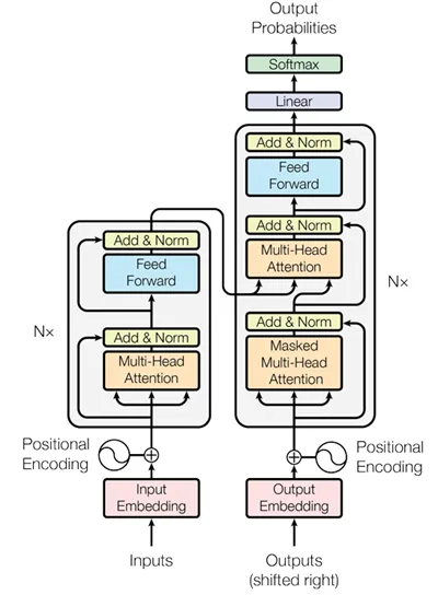
在 Transformer 网络结构中，编码器和解码器都是由多头注意力和前馈网络模块组成，在多头注意力机制中，最重要的是注意力的计算，其一般化的计算公式为：

$$\mathrm{Attention}(Q,K,V)=\mathrm{softmax}(\frac{QK^\top}{\sqrt{d_k}})V$$

其中 $Q,K,V$ 分别是查询、键、值向量。前馈网络通常由两个线性层和非线性激活组成。

在 Transformer 网络结构中共包含了三种类型的 Attention：

• Self-Attention：在 Transformer 的编码器部分，其中 $Q,K,V$ 均来自于编码器部分的输入；
• Masked Self-Attention：在 Transformer 的解码器部分，其中 $Q,K,V$ 均来自于解码器部分的输入，与 Self-Attent 不同的是，Masked Self-Attention 并不能看到所有的文本，这个在后面的计算过程部分会详细介绍到；
• Cross-Attention：这是 Transformer 的编码器和解码器结合的部分，其中 $Q$ 来自于解码器的输入，而 $K,V$ 来自于编码器的输出；

在 Self-Attention 的计算中，最重要的是 $Q,K,V$，这三者都是由输入的 Token 的向量经过线性变换得到的，我们假设 Token 的长度为 $m$，每个 Token 的维度为 $n$，输入可以表示为 $X\in \mathbb{R}^{m\times n}$，这时候有三个权重矩阵，分别为 $W_Q\in \mathbb{R}^{n\times d}$，$W_K\in \mathbb{R}^{n\times d}$ 和 $W_V\in \mathbb{R}^{n\times d}$，得到如下的线性变换的结果：

$$Q=XW_Q,\quad K=XW_K,\quad V=XW_V$$

假设此时，我们交换了输入 $X$ 的第 $i$ 行和第 $j$ 行，也就是交换了位置 $i$ 和位置 $j$ 上的词，得到 $X'$，实际上相当于左乘一个 $P\in \mathbb{R}^{m\times m}$ 矩阵，得到 $X'=PX$，其中 $P$ 具体为：

$$P=\begin{pmatrix} 1 & 0 & \cdots & 0 & \cdots & 0 & \cdots & 0 \\ 0 & 1 & \cdots & 0 & \cdots & 0 & \cdots & 0 \\ \vdots & \vdots & \cdots & \vdots &\cdots &\vdots &\cdots &\vdots \\ 0 & 0 & \cdots & 0 & \cdots & 1& \cdots &0 \\ \vdots & \vdots & \cdots & \vdots &\cdots &\vdots &\cdots &\vdots \\ 0 & 0 & \cdots & 1 & \cdots & 0& \cdots &0 \\ \vdots & \vdots & \cdots & \vdots &\cdots &\vdots &\cdots &\vdots \\ 0 & 0 & \cdots & 0 & \cdots & 0& \cdots &1 \end{pmatrix}$$

交换后，重新计算 $Q,K,V$，得到：

$$Q'=X'W_Q=PXW_Q,\quad K'=XW_K=PXW_K,\quad V'=XW_V=PXW_V$$

再计算注意力得到：

$$\begin{aligned} \mathrm{Attention}(Q',K',V') &= \mathrm{softmax}(\frac{Q'K'^\top}{\sqrt{d_k}})V'\\ & \\ &= \mathrm{softmax}(\frac{\left( PQ\right)\left(PK\right)^\top}{\sqrt{d_k}})\left(PV\right) \\ & \\ &=P\mathrm{softmax}(\frac{ QK^\top}{\sqrt{d_k}})P^T\left(PV\right) \\ &\\ &=P\mathrm{softmax}(\frac{ QK^\top}{\sqrt{d_k}})V \\ &\\ &=P\mathrm{Attention}(Q,K,V) \end{aligned}$$

这说明什么，如果只是交换了第 $i$ 行和第 $j$ 行，实际上对于最终的输出也就是交换了第 $i$ 行和第 $j$ 行。我们的目的是希望第 $i$ 个位置和 $j$ 个位置不同，这个时候就需要加入位置信息，我们注意到在 Input/Output Embedding 和 $Q,K,V$ 之间，有一个 Positional Encoding，这就是位置编码。格式为：

$$x_i = \text{TokenEmbed}(w_i) + \text{PositionEmbed}(i)$$

这个时候 $X'\neq PX$，也就没有了后面的 $\mathrm{Attention}(Q',K',V')=P\mathrm{Attention}(Q,K,V)$。

2. RoPE 被提出前位置编码的发展

最初在 Transformer^[1] 被提出的时候，为了弥补在 Self-Attention 中无法识别顺序这个问题，因此提出了位置编码的概念，在原始的 Transformer 中，使用了正弦、余弦绝对位置编码，根据位置计算固定的正弦、余弦向量，加到 Token Embedding 上。随后在 BERT^[2] 等算法中可学习绝对位置编码，每个位置有一个可训练的位置向量，与 Token Embedding 相加。在 Transformer-XL^[3] 等算法中，又提出了相对位置编码（Relative Positional Encoding），直接建模 Token 之间的相对距离。

2.1. 正弦、余弦绝对位置编码

原始 Transformer^[1]（2017）采用的就是这套方案。假设 Token 的词向量是 $x_i$，位置$i$对应的位置向量是 $PE_i$，那么输入 Transformer 的向量为 $h_i=x_i+PE_i$。

位置编码的各个维度按照不同频率计算：

$$PE_{(pos,2i)} =\sin\left(\frac{pos}{10000^{2i/d}}\right)$$

$$PE_{(pos,2i+1)} =\cos\left(\frac{pos}{10000^{2i/d}}\right)$$

其中，$pos$ 是 Token 的位置，$d$ 是 Embedding 维度。这里的位置编码是固定公式算出来的，不需要训练额外的位置参数。

2.2. 可学习绝对位置编码

BERT^[2] 等早期预训练模型采用过可学习的位置 Embedding，它与正弦位置编码的主要区别是：位置向量不是通过公式计算出来的，而是模型训练出来的参数。例如，模型最大长度为 $512$，隐藏维度为 $768$，那么可以有一个位置 Embedding 矩阵：

$$P\in\mathbb{R}^{512\times768}$$

第 $i$ 个 Token 使用：$h_i=x_i+P_i$

训练过程中，$P_i$ 和模型其他参数一起更新。

它的优点是简单直接，模型可以学习适合自身任务的位置表示；但一个局限是位置表有固定长度，超过训练或配置长度时，不能像固定公式那样直接自然地计算任意新位置。

2.3. 相对位置编码

上述的绝对位置编码告诉模型这是第几个 Token，而相对位置编码则更加关注两个 Token 之间相距多远，也就是两个 Token 的相对位置，这里面有两种，一种是 Transformer-XL^[3] 为代表的 Attention 的计算，如下：

$$A_{i,j}^{\text{rel}} = \underbrace{E_{x_i}^\top W_q^\top W_{k,E} E_{x_j}}_{(a)} + \underbrace{E_{x_i}^\top W_q^\top W_{k,R} R_{i-j}}_{(b)} + \underbrace{u^\top W_{k,E} E_{x_j}}_{(c)} + \underbrace{v^\top W_{k,R} R_{i-j}}_{(d)}$$

其中，这里的 $R_{i-j}$ 就是相对位置编码。另一种是以 T5^[4] 为代表的 Attention 的计算，一种简化形式如下：

$$\operatorname{Score}(i,j) =\frac{q_i^\top k_j}{\sqrt{d_k}}+b_{i-j}$$

其中，$b_{i-j}$ 是与相对距离相关的偏置。

3. 旋转位置编码 RoPE

旋转位置编码 RoPE^[5]，全称是 Rotary Position Embedding，是继相对位置编码后的又一位置编码形式，当前也已经成为大语言模型中非常重要的位置编码方案。在 RoPE 中，根据每一个 Token 的位置，对$Q$和$K$做旋转，让注意力分数能够体现相对位置关系。

3.1. 向量的旋转

要理解 RoPE，首先我们得看一下什么是向量的旋转，先从一个二维向量开始，假设一个二维向量 $\mathbf{x}$ 为：

$$\mathbf{x} = \begin{bmatrix} x_1\\x_2 \end{bmatrix}$$

注意：这里使用列向量是为了与旋转矩阵做矩阵运算，行向量也是可以的，相应地，计算矩阵乘积时需要对应修改旋转矩阵。

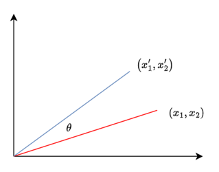
向量旋转的本质是对向量进行矩阵乘法运算，只改变向量的方向，不改变向量的大小，这个矩阵也称为旋转矩阵。这时候，我们假设这个旋转矩阵为：

$$R(\theta)= \begin{bmatrix} \cos\theta&-\sin\theta\\ \sin\theta&\cos\theta \end{bmatrix}$$

对向量进行旋矩阵乘法运算，得到：

$$\mathbf{x}'=\begin{bmatrix} x'_1\\x'_2 \end{bmatrix}=R(\theta)\mathbf{x}= \begin{bmatrix} x_1\cos\theta-x_2\sin\theta\\ x_1\sin\theta+x_2\cos\theta \end{bmatrix}$$

我们发现，旋转之后的模长没有变化，即 $\left\| \mathbf{x} \right\|=\left\| \mathbf{x}' \right\|=\sqrt{x_1^2+x_2^2}$，最终只是改变了方向，如下图所示：

对于高维的向量该如何旋转呢？推广到维度为$d$的向量，假设第 $m$ 个 Token 的维度为 $d$ 的向量为 $\mathbf{x}=[x_1,x_2,\ldots,x_d]^T$，将其拆分为 $d/2$ 个二维向量对，第 $i$ 对使用的角度为 $m\theta_i $，其中 $\theta_i$ 为：

$$\theta_i= \frac{1}{10000^{2i/d}}, i=0,1,\ldots,d/2-1$$

$m$ 表示 Token 在整个 Token 序列中的位置。最终，对于向量为 $\mathbf{x}$ 的 Token，旋转后为：

$$\mathbf{x}'=R(m\theta)\mathbf{x}$$

这就是 RoPE 的基本操作。

3.2. RoPE 与相对位置

为什么经过上面的 RoPE 后就能表示相对位置呢？要想分析 RoPE 与相对位置的关系，我们先来回顾下 Self-Attention 的计算方法，在 Transformer 中：

$$Q=XW_Q$$

$$K=XW_K$$

$$V=XW_V$$

然后计算注意力分数：

$$Attention(Q,K,V) = Softmax\left( \frac{QK^T}{\sqrt{d_k}} \right)V$$

为了方便，我们只考虑彼此的注意力分数 $QK^T$。对于任意两个 Token，假设分别是是 $m$ 个 Token 和第 $n$ 个 Token，且第 $m$ 个 Token 的 Query 向量为 $\mathbf{q}_m$，第 $n$ 个 Token 的 Key 向量为 $\mathbf{k}_n$，注意力分数为 $\mathbf{q}_m^T\mathbf{k}_n$。沿用上面的 RoPE 的计算方法，分别对 $\mathbf{q}_m$ 和 $\mathbf{k}_n$ 进行旋转：

$$\widetilde {\mathbf{q}}_m=R_m \mathbf{q}_m$$

$$\widetilde {\mathbf{k}}_n=R_n \mathbf{k}_n$$

代入注意力分数 $QK^T$，得到：

$$\begin{aligned} \widetilde {\mathbf{q}}_m^T\widetilde {\mathbf{k}}_n &= (R_m\mathbf{q}_m)^T(R_n\mathbf{k}_n)\\ & \\ &= \mathbf{q}_m^TR_m^TR_n\mathbf{k}_n \end{aligned}$$

注意：对于二维旋转矩阵，有如下的性质：

$$R(\alpha)^T=R(-\alpha)$$
$$R(\alpha)R(\beta)=R(\alpha+\beta)$$

因此，$R_m^T R_n = R(-m\theta)R(n\theta)=R((n-m)\theta)$，代入 $\widetilde {\mathbf{q}}_m^T\widetilde {\mathbf{k}}_n$ 有 $\widetilde {\mathbf{q}}_m^T\widetilde {\mathbf{k}}_n = \mathbf{q}_m^TR_{m-n}\mathbf{k}_n$。这表明，经过 RoPE 处理之后，两个 Token 的注意力分数，可以表示成一个由相对位置差$m-n$决定的旋转变换与原始 Query，Key 向量的内积。

这里需要注意的点，就是在 RoPE 中，只对 Query 和 Key 做了旋转变换，而未对 Value 有任何操作。

3.3. Llama 中的具体实现

前面对 RoPE 的原理做了简单的分析，在实际的环境中是如何使用 RoPE 的呢？我们以 Llama^[6] 中的实现为例，注意，这里只涉及到最基本的 RoPE 的实现，因为还有很多 RoPE 的改进版本。RoPE 的实现在 LlamaRotaryEmbedding 类中，在 LlamaRotaryEmbedding 类中，包含了四个方法，分别为 __init__、sin_cached、cos_cached 和 forward。

首先，__init__ 方法是整个 RoPE 机制的起点，代码如下：

def __init__(self, dim, max_position_embeddings=2048, base=10000, device=None, scaling_factor=1.0):
    super().__init__()
    self.scaling_factor = scaling_factor
    self.dim = dim
    self.max_position_embeddings = max_position_embeddings
    self.base = base
    inv_freq = 1.0 / (self.base ** (torch.arange(0, self.dim, 2, dtype=torch.int64).float().to(device) / self.dim))
    self.register_buffer("inv_freq", inv_freq, persistent=False)
    # For BC we register cos and sin cached
    self.max_seq_len_cached = max_position_embeddings
    t = torch.arange(self.max_seq_len_cached, device=device, dtype=torch.int64).type_as(self.inv_freq)
    t = t / self.scaling_factor
    freqs = torch.outer(t, self.inv_freq)
    # Different from paper, but it uses a different permutation in order to obtain the same calculation
    emb = torch.cat((freqs, freqs), dim=-1)
    self.register_buffer("_cos_cached", emb.cos().to(torch.get_default_dtype()), persistent=False)
    self.register_buffer("_sin_cached", emb.sin().to(torch.get_default_dtype()), persistent=False)

这部分代码还需要和下面的具体应用的代码结合起来一起看，程序执行中的入口函数是 forward 函数，代码如下：

@torch.no_grad()
def forward(self, x, position_ids):
    # x: [bs, num_attention_heads, seq_len, head_size]
    inv_freq_expanded = self.inv_freq[None, :, None].float().expand(position_ids.shape[0], -1, 1)
    position_ids_expanded = position_ids[:, None, :].float()
    # Force float32 since bfloat16 loses precision on long contexts
    # See https://github.com/huggingface/transformers/pull/29285
    device_type = x.device.type
    device_type = device_type if isinstance(device_type, str) and device_type != "mps" else "cpu"
    with torch.autocast(device_type=device_type, enabled=False):
        freqs = (inv_freq_expanded.float() @ position_ids_expanded.float()).transpose(1, 2)
        emb = torch.cat((freqs, freqs), dim=-1)
        cos = emb.cos()
        sin = emb.sin()
    return cos.to(dtype=x.dtype), sin.to(dtype=x.dtype)

首先是 inv_freq_expanded = self.inv_freq[None, :, None].float().expand(position_ids.shape[0], -1, 1)，这里的inv_freq是什么？其计算方法为：inv_freq = 1.0 / (self.base ** (torch.arange(0, self.dim, 2, dtype=torch.int64).float().to(device) / self.dim))，用数学形式表示就是：

$$\text{inv\_freq}[i] = \frac{1}{\text{base}^{\,\frac{2i}{dim}}}=\text{base}^{-\frac{2i}{dim}}, \quad i = 0, \dots, \frac{dim}{2}-1$$

其中，dim 为多头维度，base 通常设为 10000。这就对应了公式中 $\theta_i$ 的计算。生成的 inv_freq 是个一维的向量，向量维度为 $\frac{dim}{2}$，经过 self.inv_freq[None, :, None].float().expand(position_ids.shape[0], -1, 1) 调整维度后，inv_freq_expanded 的维度为 [batch, self.dim / 2, 1]，而 position_ids_expanded 的维度为 [Batch, 1, L]，接下来就是要计算旋转角度，freqs = (inv_freq_expanded.float() @ position_ids_expanded.float()).transpose(1, 2) 中的 @ 是 PyTorch 的矩阵乘法，用以完成二维旋转位置矩阵中 $m\theta$ 的计算，最终的维度为 [B, L, self.dim / 2]。因为这里只是计算了一半 self.dim / 2，因此需要扩展成 self.dim 维，因此就有了 emb = torch.cat((freqs, freqs), dim=-1)。最后再分别在旋转角度上做 sin 和 cos 操作。有了旋转值后，如何应用呢？有如下的函数：

def apply_rotary_pos_emb(q, k, cos, sin, position_ids=None, unsqueeze_dim=1):
    """Applies Rotary Position Embedding to the query and key tensors.

    Args:
        q (`torch.Tensor`): The query tensor.
        k (`torch.Tensor`): The key tensor.
        cos (`torch.Tensor`): The cosine part of the rotary embedding.
        sin (`torch.Tensor`): The sine part of the rotary embedding.
        position_ids (`torch.Tensor`, *optional*):
            Deprecated and unused.
        unsqueeze_dim (`int`, *optional*, defaults to 1):
            The 'unsqueeze_dim' argument specifies the dimension along which to unsqueeze cos[position_ids] and
            sin[position_ids] so that they can be properly broadcasted to the dimensions of q and k. For example, note
            that cos[position_ids] and sin[position_ids] have the shape [batch_size, seq_len, head_dim]. Then, if q and
            k have the shape [batch_size, heads, seq_len, head_dim], then setting unsqueeze_dim=1 makes
            cos[position_ids] and sin[position_ids] broadcastable to the shapes of q and k. Similarly, if q and k have
            the shape [batch_size, seq_len, heads, head_dim], then set unsqueeze_dim=2.
    Returns:
        `tuple(torch.Tensor)` comprising of the query and key tensors rotated using the Rotary Position Embedding.
    """
    cos = cos.unsqueeze(unsqueeze_dim)
    sin = sin.unsqueeze(unsqueeze_dim)
    q_embed = (q * cos) + (rotate_half(q) * sin)
    k_embed = (k * cos) + (rotate_half(k) * sin)
    return q_embed, k_embed

其中，rotate_half 函数为：

def rotate_half(x):
    """Rotates half the hidden dims of the input."""
    x1 = x[..., : x.shape[-1] // 2]
    x2 = x[..., x.shape[-1] // 2 :]
    return torch.cat((-x2, x1), dim=-1)

举个简单的例子，假设 x 为：

$$\mathbf{x}=[x_1,x_2,x_3,x_4]$$

那么，$\mathbf{x1}$ 和 $\mathbf{x2}$ 分别为：

$$\mathbf{x1}=[x_1,x_2]$$

$$\mathbf{x2}=[x_3,x_4]$$

最终，rotate_half 函数返回的是 $[-x_3, -x_4, x_1, x_2]$，代入上面的代码，得到 q_embed 和 k_embed，假设 $\mathbf{q}=[q_1,q_2,q_3,q_4]$，假设此 $\mathbf{q}$ 的旋转角度为 $[\theta_1,\theta_2,\theta_1,\theta_2]$，此时，就有：

$$\text{q\_embed}_0=q_1\times cos(\theta_1) + (-q_3)\times sin(\theta_1)$$

$$\text{q\_embed}_1=q_2\times cos(\theta_2) + (-q_4)\times sin(\theta_2)$$

$$\text{q\_embed}_2=q_3\times cos(\theta_1) + q_1\times sin(\theta_1)$$

$$\text{q\_embed}_3=q_4\times cos(\theta_2) + q_2\times sin(\theta_2)$$

```k_embed` 的计算同理。

4. 总结

在 RoPE 中通过对 Query 和 Key 进行旋转矩阵的矩阵运算后，在保持向量模长不变的情况下，自然引入了相对位置，但是 RoPE 也并不是完美的，当序列长度变得很长时，位置对应的旋转角度也会不断增大，模型可能遇到训练时未见过的位置分布，后续会有更多的改进方案来研究在长序列场景下的位置编码问题。

参考文献

[1] Vaswani A, Shazeer N, Parmar N, et al. Attention is all you need[J]. Advances in neural information processing systems, 2017, 30.

[2] Devlin J , Chang M W , Lee K , et al. BERT: Pre-training of Deep Bidirectional Transformers for Language Understanding[J]. 2018.

[3] Dai Z, Yang Z, Yang Y, et al. Transformer-xl: Attentive language models beyond a fixed-length context[C]//Proceedings of the 57th annual meeting of the association for computational linguistics. 2019: 2978-2988.

[4] Raffel C, Shazeer N, Roberts A, et al. Exploring the limits of transfer learning with a unified text-to-text transformer[J]. Journal of machine learning research, 2020, 21(140): 1-67.

[5] Su J, Ahmed M, Lu Y, et al. Roformer: Enhanced transformer with rotary position embedding[J]. Neurocomputing, 2024, 568: 127063.

[6] Llama 代码中的 RoPE